From Linear Regression to Neural Networks

These days there exists much hype around sophisticated machine learning methods such as Neural Networks — they are massively powerful models that allow us to fit very flexible models. However, we do not always require the full complexity of a Neural Network: sometimes, a simpler model will do the job just fine. In this project, we take a journey starting from the most fundamental statistical machinery to model data distributions, linear regression, to then explain the benefits of constructing more complex models, such as logistic regression or a Neural Network. In this way, this text aims to build a bridge from the statistical, analytical world to the more approximative world of Machine Learning. We will not shy away from the math, whilst still working with tangible examples at all times: we will work with real-world datasets and we will get to apply our models as we go on. Let's start!

Linear Regression (Code)

First, we will explore linear regression, for it is an easy to understand model upon which we can build more sophisticated concepts. We will use a dataset on Antarctican penguins (Gorman et al., 2014) to conduct a regression between the penguin flipper length as independent variable $X$ and the penguin body mass as the dependent variable $Y$. We can analytically solve Linear Regression by minimizing the Residual Sum-of-Squares cost function (Hastie et al., 2009):

$$\text{R}(\beta) = (Y - X \beta)^T (Y - X \beta)$$

In which $X$ is our design matrix. Regression using this loss function is also referred to as "Ordinary Least Squares". The mean of the cost function $\text{R}$ over all samples is called Mean Squared Error, or MSE. Our design matrix is built by appending each data row with a bias constant of 1 - an alternative would be to first center our data to get rid of the intercept entirely. To now minimize our cost function we differentiate $\text{R}$ with respect to $\beta$, giving us the following unique minimum:

$$\hat{\beta} = (X^T X)^{-1} X^T Y$$

... which results in the estimated least-squares coefficients given the training data, also called the normal equation. We can classify by simply multiplying our input data with the found coefficient matrix: $\hat{Y} = X \hat{\beta}$. Let's observe our fitted regression line onto the data:

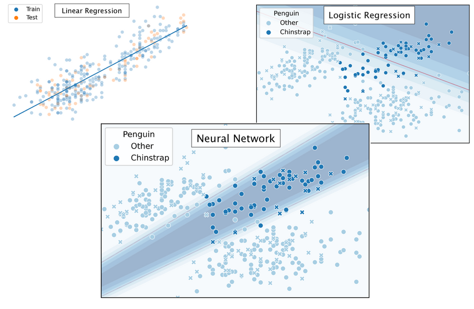
We can observe visually that our estimator explains both the training and testing data reasonably well: the line positioned itself along the mean of the data. This is in fact the proposition we make in least-squares - we assume the target to be Gaussian distributed; which in the case of modeling this natural phenomenon, penguins, seems to fit quite well.

Because at the moment we are very curious, we would also like to explore using a more flexible model. Note that our normal equation we defined above tries to find whatever parameters make the system of linear equations produce the best predictions on our target variable. This means, that hypothetically, we could add any linear combination of explanatory variables we like: such create estimators of a higher-order polynomial form. This is called polynomial regression. To illustrate, a design matrix for one explanatory variable $X_1$ would look as follows:

$$X= \left[\begin{array}{ccccc}1 & x_{1} & x_{1}^{2} & \ldots & x_{1}^{d} \\ 1 & x_{2} & x_{2}^{2} & \ldots & x_{2}^{d} \\ 1 & x_{3} & x_{3}^{2} & \ldots & x_{3}^{d} \\ \vdots & \vdots & \vdots & \ddots & \vdots \\ 1 & x_{n} & x_{n}^{2} & \ldots & x_{n}^{d}\end{array}\right]$$

Which results in $d$-th degree polynomial regression. The case $d=1$ is just normal linear regression. For example sake, let us sample only $n=10$ samples from our training dataset, and try to fit those with a polynomial regressors of increasing degrees. Let us observe what happens to the training and testing loss accordingly:

It can be observed that although for some degrees the losses remain almost the same, we suffer from overfitting after the degree passes $d=30$. We can also visually show how the polynomials of varying degrees fit our data:

We can indeed observe that the polynomials of higher degree definitely do not better explain our data. Also, the polynomials tend to get rather erratic beyond the last data points of the training data - which is important to consider whenever predicting outside the training data value ranges. Generally, polynomials of exceedingly high degree can overfit too easily and should only be considered in very special cases.

Up till now our experiments have been relatively simple - we used only one explanatory and one response variable. Let us now explore an example in which we use all available explanatory variables to predict body mass, to see whether we can achieve an even better fit. Because we are now at risk of suffering from multicolinearity; the situation where multiple explanatory variables are highly linearly related to each other, we will use an extension of linear regression which can deal with such a situation. The technique is called Ridge Regression.

Ridge Regression

In Ridge Regression, we aim to tamper the least squares tendency to get as 'flexible' as possible to fit the data best it can. This might, however, cause parameters to get very large. We therefore like to add a penalty on the regression parameters $\beta$; we penalise the loss function with a square of the parameter vector $\beta$ scaled by new hyperparameter $\lambda$. This is called a shrinkage method, or also: regularization. This causes the squared loss function to become:

$$\text{R}(\beta) = (Y - X \beta)^T (Y - X \beta)+\lambda \beta^T \beta$$

This is called regularization with an $L^2$ norm; which generalization is called Tikhonov regularization, which allows for the case where not every parameter scalar is regularized equally. If we were to use an $L^1$ norm instead, we would speak of LASSO regression. If we were to now derive the solutions of $\beta$ given this new cost function by differentiation w.r.t. $\beta$:

$$\hat{\beta}^{\text {ridge }}=\left(\mathbf{X}^{T} \mathbf{X}+\lambda \mathbf{I}\right)^{-1} \mathbf{X}^{T} \mathbf{Y}$$

In which $\lambda$ will be a scaling constant that controls the amount of regularization that is applied. Note $\mathbf{I}$ is the $p\times p$ identity matrix - in which $p$ are the amount of data dimensions used. An important intuition to be known about Ridge Regression, is that directions in the column space of $X$ with small variance will be shrinked the most; this behavior can be easily shown be deconstructing the least-squares fitted vector using a Singular Value Decomposition. That said, let us see whether we can benefit from this new technique in our experiment.

In the next experiment, we will now use all available quantitative variables to try and predict the Penguin body mass. The Penguin- bill length, bill depth and flipper length will be used as independent variables. Note, however, they might be somewhat correlated: see this pairplot on the Penguin data for details. This poses an interesting challenge for our regression. Let us combine this with varying dataset sample sizes and varying settings of $\lambda$ to see the effects on our loss.

Ridge Regression using all quantitative variables in the Penguin dataset to predict body mass. Varying subset sizes of the dataset $n$ as well as different regularization strengths $\lambda$ are shown.

It can be observed, that using including all quantitative variables did improve the loss on predicting the Penguin body mass using Ridge Regression. In fact, the penalty imposed probably pulled the hyperplane angle down such that the error in fact increased. Ridge Regression is a very powerful technique, nonetheless, and most importantly introduced us to the concept of regularization. In the next chapters on Logistic Regression in Neural Networks, we assume all our models to use $L^2$ regularization.

Now, the data we fit up until now had only a small dimensionality - this is perhaps a drastic oversimplification in comparison to the real world. How does the analytic way of solving linear regression using the normal equation fare with higher-dimensional data?

High-dimensional data

In the real world, datasets might be of very high dimensionality: think of images, speech, or a biomedical dataset storing DNA sequences. These datasets cause different computational strain on the equations to be solved to fit a linear regression model: so let us simulate such a high-dimensional situation.

In our simulation the amount of dimensions will configured to outmatch the amount of dataset samples ($p \gg n$), which extra dimensions we will create by simply adding some noise columns to the design matrix $X$. The noise will be drawn from a Gaussian distribution $\epsilon \sim \mathcal{N}(0, 1)$. We can now run an experiment by fitting our linear regression model to the higher-dimensional noised dataset, benchmarking the fitting times of the algorithm.

We can observe that the normal equation takes a lot longer to compute for higher-dimensional data. In fact, numerically computing the matrix inverse is very computationally expensive, i.e. computing $(X^TX)^{-1}$. Luckily, there are computationally cheaper techniques to do a regression in higher-dimensional spaces. One such technique is an iterative procedure, called Gradient Descent.

Gradient Descent

Instead of trying to analytically solve the system of linear equations at once, we can choose an iterative procedure instead, such as Gradient Descent. It works by computing the gradient of the cost function with respect to the model weights - such that we can then move in the opposite direction of the gradient in parameter space. Given some loss function $R(\beta)$ and $R_i(\beta)$, which computes the empirical loss for entire dataset and for the $i$-th observation, respectively, we can define one gradient descent step as:

$$\begin{aligned} \beta^{(r + 1)} &= \beta^{(r)} - \gamma \nabla_{\beta^{(r)}} R(\beta^{(r)}) \\ &= \beta^{(r)} - \gamma \sum_{i=1}^N \frac{\partial R_i(\beta^{(r)})}{\partial \beta^{(r)}}\\ \end{aligned}$$

In which $\gamma$ is the learning rate and $r$ indicates some iteration - given some initial parameters $\beta^0$ and $N$ training samples. Using this equation, we are able to reduce the loss in every iteration, until we converge. Convergence occurs when every element of the gradient is zero - or very close to it. Although gradient descent is used in this vanilla form, two modifications are common: (1) subsampling and  using a (2) learning rate schedule.

1. Although in a scenario in which our loss function landscape is convex the vanilla variant does converge toward the global optimum relatively easily, this might not be the case for non-convex error landscapes. We are at risk of getting stuck in local extremes. In this case, it is desirable to introduce some randomness — allowing us to jump out local extrema. We can introduce randomness by instead of computing the gradient over the entire sample set, we can do so for a random sample of the dataset called a minibatch (Goodfellow et al., 2014). A side effect is a lighter computational burden per iteration; sometimes causing faster convergence. Because the introduced randomness makes the procedure stochastic instead of deterministic, we call this algorithm Stochastic Gradient Descent, or simply SGD.
2. Accommodating SGD is often a learning rate schedule: making the learning rate parameter $\gamma$ dependent on the iteration number $r$ such that $\gamma = \gamma^{(r)}$. In this way, we made the learning rate adaptive over time, allowing us to create a custom learning rate scheme. Many schemes (Dogo et al., 2018) exist - which can be used to avoid spending a long time on flat areas in the error landscape called plateaus, or to avoid 'overshooting' the optimal solution. Even, a technique analogous with momentum (Qian, 1999) in physics might be used: a particle traveling through space is 'accelerated' by the loss gradient, causing the gradient to change faster if it keeps going in the same direction.

So, let's now redefine our gradient descent formula to accommodate for these modifications:

$$\beta^{(r+1)}=\beta^{(r)}-\gamma^{(r)} \frac{1}{m} \sum_{i=1}^m \frac{\partial R_i(\beta^{(r)})}{\partial \beta^{(r)}} $$

... where we, before each iteration, randomly shuffle our training dataset such that we draw $m$ random samples each step. The variable $m$ denotes the batch size - which can be anywhere between 1 and the amount of dataset samples minus one $N - 1$. The smaller the batch size, the more stochastic the procedure will get.

Using gradient descent for our linear regression is straight-forward. We differentiate the cost function with respect to the weights; the least squares derivative is then as follows:

$$\begin{aligned} \frac{\partial R_i(\beta^{(r)})}{\partial \beta^{(r)}} &= \frac{\partial}{\partial \beta^{(r)}} (y_i - x_i \beta^{(r)})^2\\ &= 2 (y_i - x_i \beta^{(r)})\\ \end{aligned}$$

We then run the algorithm in a loop, to iteratively get closer to the optimum parameter values.

Now, using this newly introduced iterative optimization procedure, let's see whether we can solve linear regression faster. First, we will compare SGD and the analytic method for our Penguin dataset with standard Gaussian noise dimensions added such that $p=2000$.

Indeed - our iterative procedure is faster for such a high-dimensional dataset. Because the analytic method always finds the optimum value, it is most plausible that SGD does not achieve the same performance - as can be seen in the MSE loss in the figure. Only in a couple of runs does SGD achieve near-optimum performance - in the other cases the algorithm was either stopped by its maximum iterations limit or it got stuck in some local extrema and has not gotten out yet. If we wanted to get better results, we could have used a more lenient maximum amount of iterations or a stricter convergence condition. This is a clear trade-off between computational workload and the optimality of the solution. We can run some more experiments for various levels of augmented dimensions:

In which we can empirically show that for our experiment, the analytic computation time grows about exponentially whilst SGD causes only a mild increase in computational time. SGD does suffer a higher loss due to its approximative nature - but this might just be worth the trade-off.

Now that we have gotten familiar with Gradient Descent, we can explore a realm of techniques that rely on being solved iteratively. Instead of doing regression, we will now try to classify penguins by their species type — a method for doing so is Logistic Regression.

Logistic Regression (Code)

In general, linear regression is no good for classification. There is no notion incorporated into the objective function to desire a hyperplane that best separates two classes. Even if we would encode qualitative target variables in a quantitative way, i.e. in zeros or ones, a normal equation fit would result in predicted values outside the target range.

Therefore, we require a different scheme. In Logistic Regression, we first want to make sure all estimations remain in $[0,1]$. This can be done using the Sigmoid function:

$$S(z)=\frac{e^z}{e^z+1}=\frac{1}{1+e^{-z}}$$

Also called the Logistic function. So, the goal is to predict some class $G \in \{1,\dots,K\}$ given inputs $X$. We assume an intercept constant of 1 to be embedded in $X$. Now let us take a closer look at the case where $K=2$, i.e. the binary or binomial case.

If we were to encode our class targets $Y$ as either ones or zeros, i.e. $Y \in \{0,1\}$, we can predict values using $X \beta$ and pull them through a sigmoid $S(X\beta)$ to obtain the probabilities whether samples belongs to the class encoded as 1. This can be written as:

$$\begin{aligned} \Pr(G=2|X;\beta)&=S(X\beta)\\ &=\frac{1}{1+\exp(-X\beta)}\\ &=p(X;\beta) \end{aligned}$$

Because we consider only two classes, we can compute one probability and infer the other one, like so:

$$\begin{aligned} \Pr(G=1|X;\beta)&=1-p(X;\beta) \end{aligned}$$

For which it can be easily seen that both probabilities form a probability vector, i.e. their values sum to 1. Note we can consider the targets as a sequence of Bernoulli trials $y_i,\dots,y_N$ - each outcome a binary - assuming all observations are independent of one another. This allows us to write:

$$\begin{aligned} \Pr (y| X;\beta)&=p(X;\beta)^y(1-p(X;\beta))^{(1-y)}\\ \end{aligned}$$

So, how to approximate $\beta$? Like in linear regression, we can optimize a loss function to obtain an estimator $\hat{\beta}$. We can express the loss function as a likelihood using Maximum Likelihood Estimation. First, we express our objective into a conditional likelihood function.

$$\begin{aligned} L(\beta)&=\Pr (Y| X;\beta)\\ &=\prod_{i=1}^N \Pr (y_i|X=x_i;\beta)\\ &=\prod_{i=1}^N p(x_i;\beta)^{y_i}(1-p(x_i;\beta))^{(1-y_i)} \end{aligned}$$

The likelihood becomes easier to maximize in practice if we rewrite the product to a sum using a logarithm; such scaling does not change the resulting parameters. We obtain the log-likelihood (Bischop, 2006):

$$\begin{aligned} \ell(\beta)&=\log L(\beta)\\ &=\sum_{i=1}^{N}\left\{y_{i} \log p\left(x_{i} ; \beta\right)+\left(1-y_{i}\right) \log \left(1-p\left(x_{i} ; \beta\right)\right)\right\}\\ &=\sum_{i=1}^{N}\left\{y_{i} \beta^{T} x_{i}-\log \left(1+e^{\beta^{T} x_{i}}\right)\right\} \end{aligned}$$

Also called the logistic loss; which multi-dimensional counterpart is the cross-entropy loss. We can maximize this likelihood function by computing its gradient:

$$\frac{\partial \ell(\beta)}{\partial \beta}=\sum_{i=1}^{N} x_{i}\left(y_{i}-p\left(x_{i} ; \beta\right)\right)$$

...resulting in $p+1$ equations nonlinear in $\beta$. The equation is transcendental: meaning no closed-form solution exists and hence we cannot simply solve for zero. It is possible, however, to use numerical approximations: Newton-Raphson method based strategies can be used, such as Newton Conjugate-Gradient, or quasi-Newton procedures might be used such as L-BFGS (Zhu et al., 1997). Different strategies have varying benefits based on the problem type, e.g. the amount of samples $n$ or dimensions $p$. Since the gradient can be approximated just fine, we can also simply use Gradient Descent, i.e. SGD.

In the case where more response variables are to be predicted, i.e. $K>2$, a multinomial variant of Logistic Regression can be used. For easier implementation, some software implementations just perform multiple binomial logistic regressions in order to conduct a multinomial one; which is called a One-versus-All strategy. The resulting probabilities are then normalized to still output a probability vector (Pedregosa et al., 2001).

That theory out of the way, let's fit a Logistic Regression model to our penguin data! We will try to classify whether a penguin is a Chinstrap yes or no, in other words: we will perform a binomial logistic regression. We will perform 30K iterations, each iteration an epoch over the training data:

We can observe that the model converged to a stable state already after about 10K epochs - we could have implemented an early stopping rule; for example by checking whether validation scores stop improving or when our loss is no longer changing much. We can also visualize our model fit over time: by predicting over a grid of values at every time step during training. This yields the following animation:

Clearly, our decision boundary is not optimal yet - whilst the data is somewhat Gaussian distributed our model linearly separates the data. We can do better — we need some way to introduce more non-linearity into our model. A model that does just so is a Neural Network.

Neural Network (Code)

At last, we arrive at the Neural Network. Using the previously learned concepts, we are really not that far off from assembling a Neural Network. Really, a single-layer Neural Network essentially just a linear model, like before. The difference is, that we conduct some extra projections in order to make the data better linearly separable. In a Neural Network, we aim to find the parameters facilitating such projections automatically. We call each such projection a Hidden Layer. After having conducted a suitable projection,  we can pull the projected data through a logistic function to estimate a probability - similarly to logistic regression. One such architecture is like so:

So, given one input vector $x_i$, we can compute its estimated value by feeding its values through the network from left to right, in each layer multiplying with its parameter vector. We call this type of network feed-forward. Networks that do not feed forward include recurrent or recursive networks, though we will only concern ourselves with feed-forward networks for now.

An essential component of any such network is an activation function; a non-linear differentiable function mapping $\mathbb{R} \rightarrow \mathbb{R}$, aimed to overcome model linearity constraints. We apply the activation function to every hidden node; we compute the total input, add a bias, and then activate. This process is somewhat analogous to what happens in neurons in the brain - hence the name Neural Network. Among many possible activation functions (Nwankpa et al., 2018), a popular choice is the Rectified Linear Unit, or ReLU: $\sigma(z)=\max\{0, z\}$. It looks as follows:

Also because ReLU is just a max operation, it is fast to compute (e.g. compared to a sigmoid). Using our activation function, we can define a forward-pass through our network, as follows:

$$\begin{aligned} h^{(1)}&=\sigma(X W^{(1)} + b^{(1)})\\ h^{(2)}&=\sigma(h^{(1)} W^{(2)} + b^{(2)})\\ h^{(3)}&=\sigma(h^{(2)} W^{(3)} + b^{(3)})\\ \hat{Y}&=S(h^{(3)}W^{(4)}+b^{(4)}) \end{aligned}$$

In which $h$ resembles the intermediate projections indexed by its hidden layer; and the parameters $\beta$ mapping every two layers together are accessible through $W$. A bias vector is accessible through $b$, such to add a bias term to every node in the layer. Finally, we apply a Sigmoid to the results of the last layer to receive probability estimates; in the case of multi-class outputs its multi-dimensional counterpart is used, the Softmax, which normalizes the logistic function such to produce a probability vector. Do note that the activation function could differ per layer; and in practice, this might happen. In our case, we will just use one activation function for all hidden layers in our network.

We are also going to have to define a cost function, such to be able to optimize the parameters based on its gradient. We can do so using the minimizing the negative log-likelihood using Maximum Likelihood, given some loss function such as:

$$ R(\theta)=-\mathbb{E}_{\mathbf{x}, \mathbf{y}\sim\hat{p}_{\text{data }}}\log p_{\operatorname{model}}(\boldsymbol{y}\mid\boldsymbol{x}) $$

In which we combined weights $W$ and biases $b$ into a single parameter term $\theta$. Our cost function says to quantify the chance of encountering a target $y$ given an input vector $x$. Suitable loss functions to be used are log-loss/cross-entropy, or simply squared error:

$$ R(\theta)=\frac{1}{2}\mathbb{E}_{\mathbf{x}, \mathbf{y}\sim\hat{p}_{\text{data }}}\|\boldsymbol{y}-f(\boldsymbol{x} ; \boldsymbol{\theta})\|^{2}+ \text{const} $$

Assuming $p_{\text{model}}(y|x)$ to be Gaussian distributed. Of course, in any implementation we can only approach the expected value by averaging over a discrete set of observations; thus allowing us to compute the loss of our network.

Now that we are able to do a forward pass by (1) making predictions given a set of parameters $\theta$ and (2) computing its loss using a cost function $R(\theta)$, we will have to figure out how to actually train our network. Because our computation involves quite some operations by now, computing the gradient of the cost function is not trivial - to approximate the full gradient one would have to compute partial derivatives with respect to every weight separately. Luckily, we can exploit the calculus chain rule to break up the problem into smaller pieces: allowing us to much more efficiently re-use previously computed answers. The algorithm using this trick is called back-propagation.

In back-propagation, we re-visit the network in reverse order; i.e. starting at the output layer and working our way back to the input layer. We then use the calculus derivative chain rule (Goodfellow et al., 2014):

$$\begin{aligned} \frac{\partial z}{\partial x_{i}}&=\sum_{j} \frac{\partial z}{\partial y_{j}} \frac{\partial y_{j}}{\partial x_{i}}\\ &\text{in vector notation:}\\ \nabla_{\boldsymbol{x}} z&=\left(\frac{\partial \boldsymbol{y}}{\partial \boldsymbol{x}}\right)^{\top} \nabla_{\boldsymbol{y}} z \end{aligned}$$

...to compute the gradient in modular fashion. Note we need to consider the network in its entirety when computing the partial derivatives; the output activation, the loss function, node activations and the biases. To systematically apply back-prop to a network often these functions are abstracted as being an operation - which can then be assembled in a computational graph. Given a suitable such graph, many generic back-prop implementations can be used.

Once we have now computed the derivative of the cost function $R(\theta)$, our situation became similar to when we iteratively solved linear- or logistic regression: we can now use just Gradient Descent to move in the error landscape.

Now that we know how to train a Neural Network, let's apply it! We aim to get better accuracy for our Penguin classification problem than using our Logistic Regression model.

Indeed, our more flexible Neural Network model better fits the data. The NN achieves 94.9% testing accuracy, in comparison to 89.7% testing accuracy for the Logistic Regression model. Let's see how our model is fitted over time:

In which it can be observed that the model converged after some 750 iterations. Intuitively, the decision region looks to have been approximated fairly well - it might just have been slightly 'stretched' out.

Ending note

Now that we have been able to fit a more 'complicated' data distribution, we conclude our journey from simple statistical models such a linear regression up to Neural Networks. Having a diverse set of statistical and iterative techniques in your tool belt is essential for any Machine Learning practitioner: even though immensely powerful models are available and widespread today, sometimes a simpler model will do just fine.

In tandem with how the bias/variance dilemma is fundamental to understanding how to construct good distribution learning models, one should always take into account not to overreach on model complexity given a learning task (Occam's Razor; Rasmussen et al., 2001): use an as simple as possible model, wherever possible.

Citations

• Gorman KB, Williams TD, Fraser WR (2014). Ecological sexual dimorphism and environmental variability within a community of Antarctic penguins (genus Pygoscelis). PLoS ONE 9(3):e90081.
• Hastie, T., Tibshirani, R., & Friedman, J. (2009). The elements of statistical learning: data mining, inference, and prediction. Springer Science & Business Media.
• Dogo, E. M., Afolabi, O. J., Nwulu, N. I., Twala, B., & Aigbavboa, C. O. (2018, December). A comparative analysis of gradient descent-based optimization algorithms on convolutional neural networks. In 2018 International Conference on Computational Techniques, Electronics and Mechanical Systems (CTEMS) (pp. 92-99). IEEE.
• Bishop, C. M. (2006). Pattern Recognition and Machine Learning. Springer.
• Goodfellow, I., Bengio, Y., Courville, A., & Bengio, Y. (2016). Deep learning (Vol. 1, No. 2). Cambridge: MIT press.
• Qian, N. (1999). On the momentum term in gradient descent learning algorithms. Neural networks, 12(1), 145-151.
• Zhu, C., Byrd, R. H., Lu, P., & Nocedal, J. (1997). Algorithm 778: L-BFGS-B: Fortran subroutines for large-scale bound-constrained optimization. ACM Transactions on Mathematical Software (TOMS), 23(4), 550-560.
• Pedregosa, F., Varoquaux, G., Gramfort, A., Michel, V., Thirion, B., Grisel, O., ... & Duchesnay, E. (2011). Scikit-learn: Machine learning in Python. the Journal of machine Learning research, 12, 2825-2830.
• Nwankpa, C., Ijomah, W., Gachagan, A., & Marshall, S. (2018). Activation functions: Comparison of trends in practice and research for deep learning. arXiv preprint arXiv:1811.03378.
• Rasmussen, C. E., & Ghahramani, Z. (2001). Occam's razor. Advances in neural information processing systems, 294-300.

Code

The code is freely available on Github, see: